Variational Inference with Node Embeddings (VINE)
Siepel, Hassett, Staklinski — bioRxiv 2025
McCrone Lab Meeting
2025-01-08
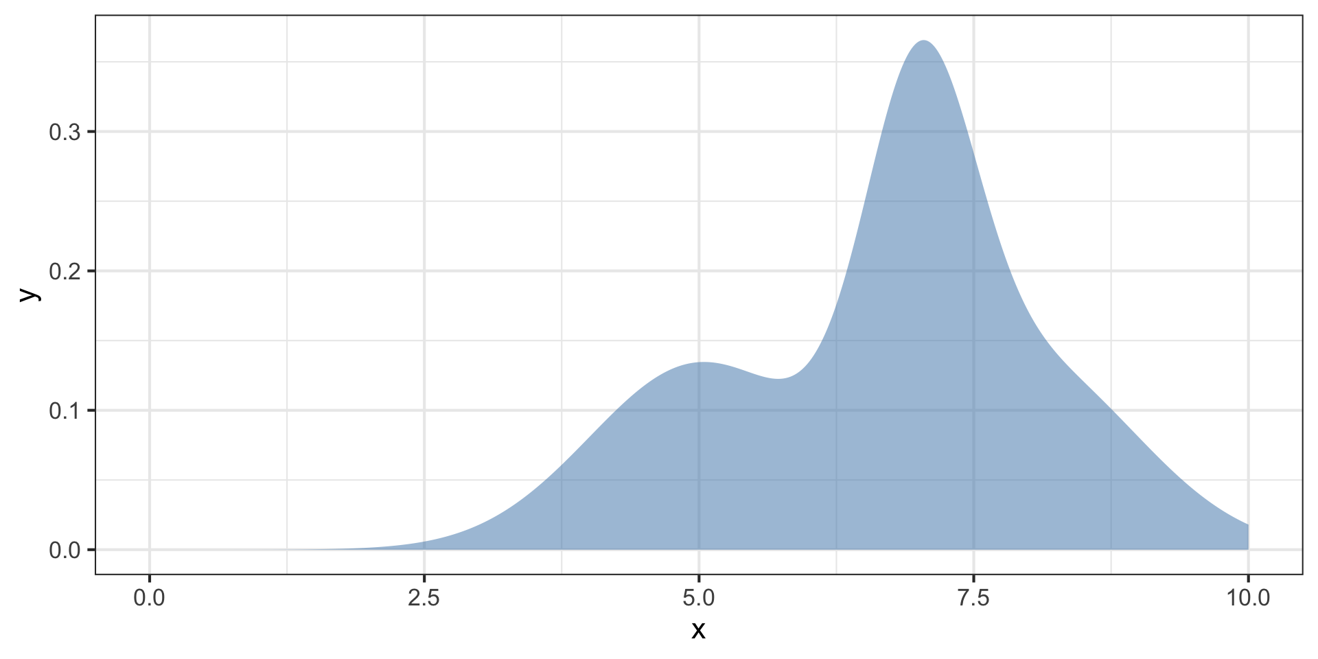
Posterior distributions are hard to characterize
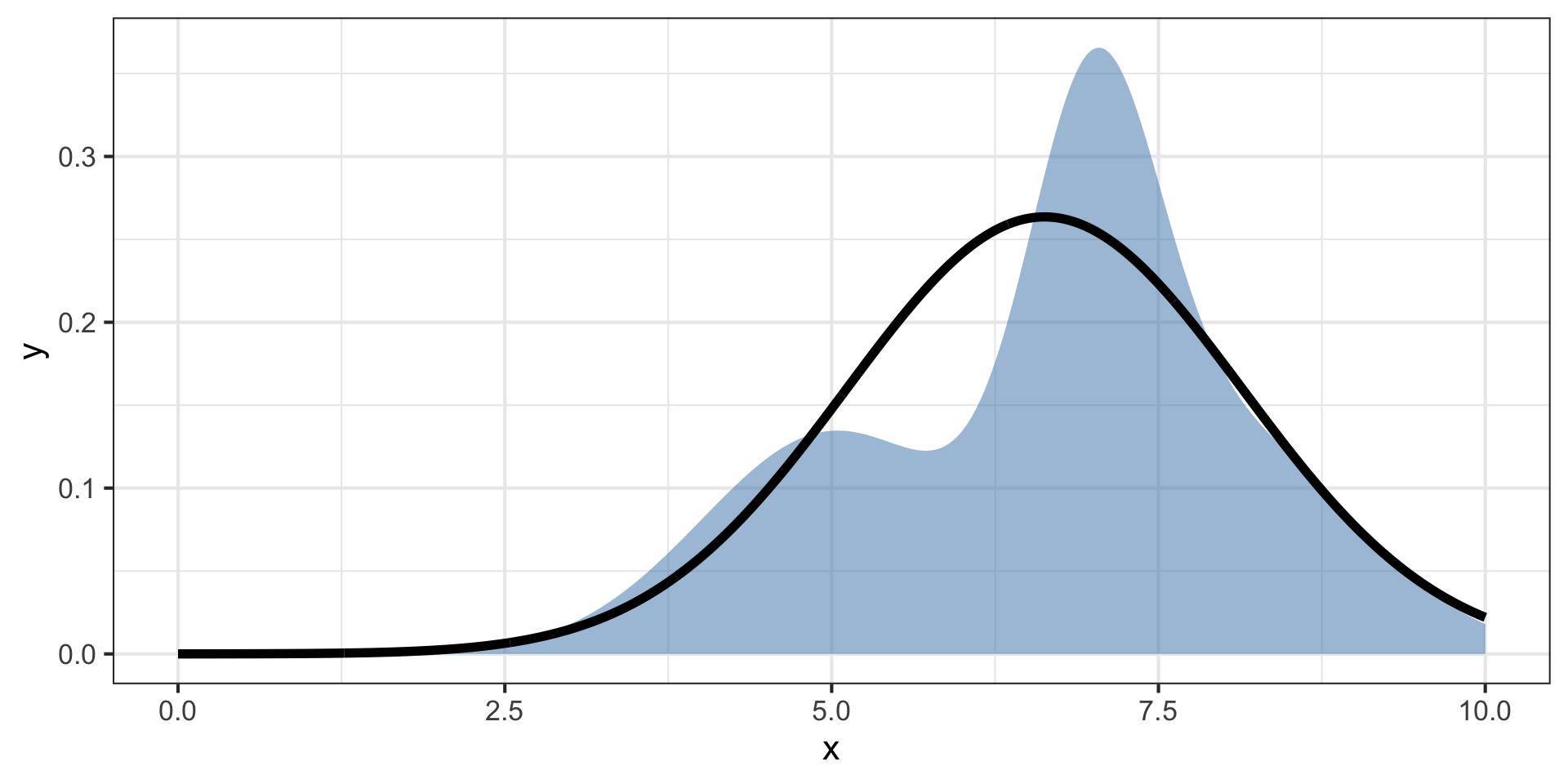
We can use another function \(q(z)\) to approximate the posterior \(p(x,z)\).
This is variational inference (VI)
Posterior distributions are hard to characterize
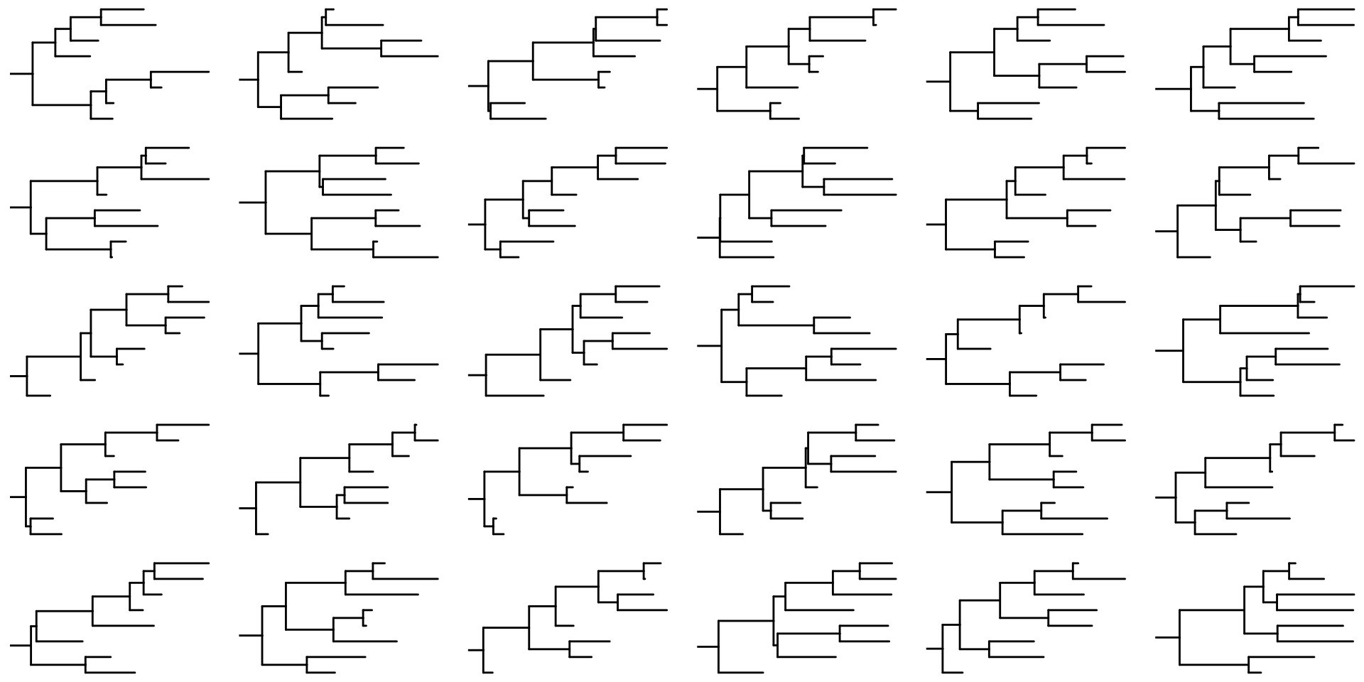
What if we could approximate the distribution of topologies and branch lengths with another distribution?
The central problem for VI on trees
Approximate the Bayesian posterior distribution of trees given a set of observed genotypes \(\mathbf{X}\) using a variational distribution \(q(\tau, \mathbf{b}; \theta)\)
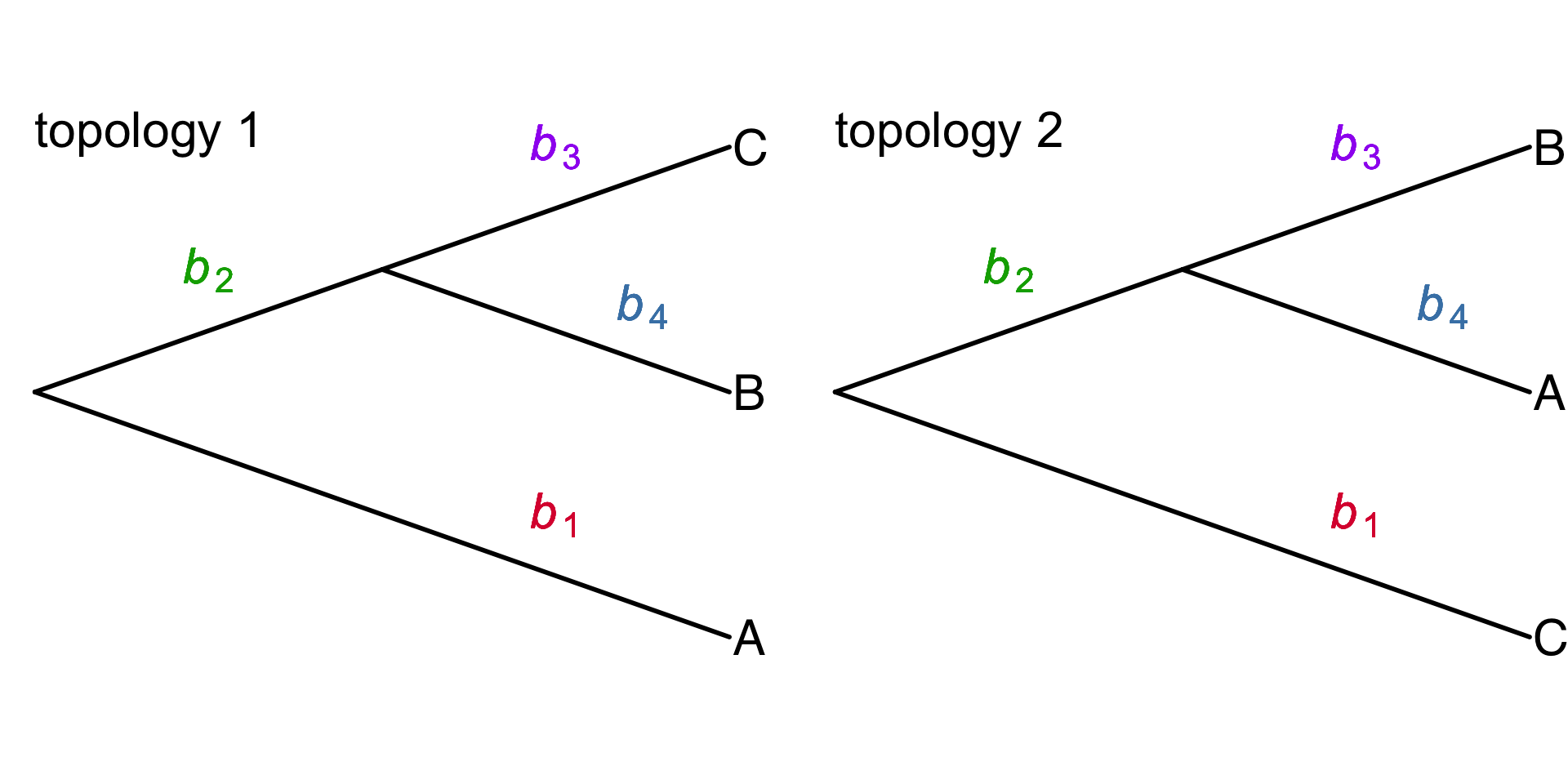
\(\tau\) – topology of a tree
\(\mathbf{b}\) – vector of branch lengths
\([\)\(b_1\), \(b_2\), \(b_3\), \(b_4\)\(]\)
\(\theta\) – free parameters of the variational distribution
Typically, \(q\) is fitted to data by adjusting \(\theta\) to minimize the KL divergence from the true posterior distribution \(p(\tau,\mathbf{b} \mid X)\)
VINE steps
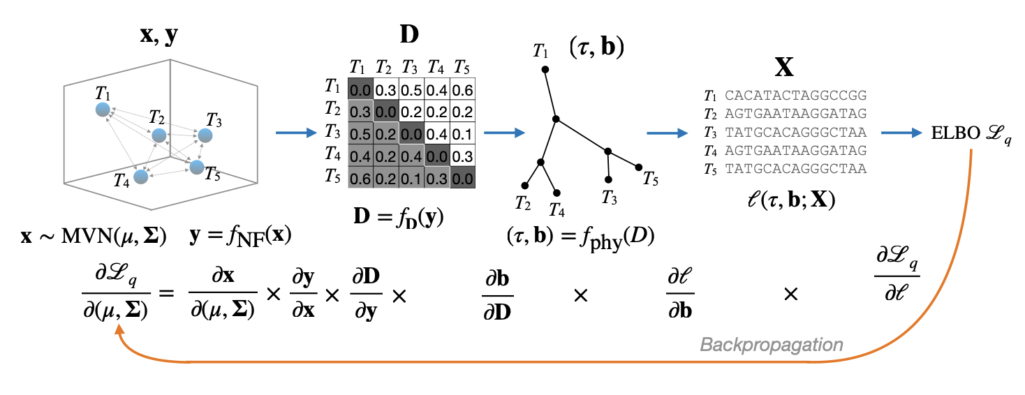
- Embedding – parameterized using a multivariate normal (\(\mathbb{R}^5\))
- Distance matrix is induced from the embedding
- Converted to a tree using neighbor joining
- Compute the likelihood of the branch lengths and topology given the sequences
- MCMC or Taylor Approximation of the ELBO (Evidence lower bound)